4.1 Parametric Functions

4.1 Parametric Functions

A parametric function in R^2 is a way to represent a curve or a surface in a two-dimensional space using a set of two equations. These equations are called parametric equations, and they express the values of the two dependent variables x and y as functions of the independent variable t. 🎨

Source: Stony Brook

👌 Advantages

One of the main advantages of using parametric functions is that it allows for a more flexible representation of the geometric objects. 🤸 For example, a parametric function can represent a circle, an ellipse, a parabola, or a hyperbola, all with the same set of equations, depending on the values of the parameters. 🌀

Also, it can represent more complex shapes, such as helixes, tori, and other geometric objects that can't be represented by a single algebraic equation. 💎

Another advantage of parametric functions is that it can be easily used to create animations and interactive graphics. By varying the value of the parameter, we can create a dynamic representation of the curve or surface, which can be useful in fields such as computer graphics and engineering design. 🧑‍💻

⚙️ Mechanics

The coordinates of a point in the R^2 plane, (x_i, y_i), at a specific value of the parameter, t_i, can be written as functions of t. This can be expressed as the single parametric function f(t) = (x(t), y(t)), where x(t) and y(t) are the two functions that represent the coordinates of a point in the R^2 plane at any value of the parameter t. 📝

This way of representing a curve, known as a parametric representation, allows for a more general and versatile way of describing a curve in the R^2 plane. It is particularly useful when the curve does not have a simple equation in terms of x and y, such as the case of circles or ellipses.

Parametric representation also allows for the representation of more complex curves such as spirals, cycloids, and epicycloids, which cannot be represented by simple algebraic equations. 〽️ Additionally, the use of a parameter in the parametric representation allows for the animation of the curve, providing a dynamic visualization of the movement of the curve. It also allows for the easy calculation of the curve's length and the calculation of tangents and normals. 😲

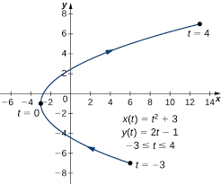
Source: Math LibreTexts

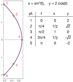
A numerical table of values can be generated for the parametric function f(t) = (x(t), y(t)) by evaluating x_i and y_i at several values of t_i within the domain of the function. #️⃣ This allows for the visual representation of the function in the form of a graph, which can be useful in understanding the behavior of the function and identifying any patterns or characteristics. 🪑

Source: Xaktly

One example of a parametric function is the representation of a point on a circle. A circle with center (h, k) and radius r can be represented by the parametric equations x(t) = h + rcos(t) and y(t) = k + rsin(t). By varying the value of t, we can trace the point on the circle as it moves around the circumference. This representation allows for a convenient way to analyze the motion of a point on a circle and understand the relationship between the angle and the coordinates of the point. 🔵

🌟 Domains

The domain of the parametric function f is often restricted, which results in start and end points on the graph of f. This is because the parameter, t, is only allowed to take on certain values within a specified range (known as the domain of the function). 🙅

For example, if the domain of the function is defined as 0 < t < π, then the parameter t can only take on values between 0 and pi. As a result, the graph of the function will only be defined within this range and will have start and end points at the values of t where the domain begins and ends. These points are known as the start and end points of the parametric curve. 🛑

The graph of the function can be visualized by plotting the x and y coordinates for each value of t within the domain and connecting the points to form a continuous curve. By understanding the domain of the function, we can better understand the shape, location and extent of the graph of the function. ♠️